Mean Shift
1. Kernel Density Estimation
Kernel density estimation(KDE) is a non-parametric method to estimate the probability density function(pdf). A non-parametric density estimator assumes no pre-specified function form for the pdf. Assume \(X = (x_1, x_2, ... x_n), x_i \in \mathbf{R}^d\) are independent and identically distributed(i.i.d.) random variables with continuous density function \(f\), the kernel density estimator is defined as
\[\begin{equation} \hat{f}(x;H)= \sum_{i=1}^{n} \alpha_i \mathbf{K}(x-x_i, H) \label{eq1} \end{equation}\]where \(\mathbf{K}\) is the kernel, \(H\) is the bandwidth, and \(\alpha_i\) is the weighting coefficient.
1.1 Interpretation
In my understanding, the form of equation \(\eqref{eq1}\) can be interpreted like this:
-
The kernel \(K_i = K(x-x_i, H)\) is the estimated density function for data point \(x_i\)
-
The coefficient \(\alpha_i\) is the weight for data point \(x_i\), usually set as \(1/n\)
-
\(\sum_{i=1}^{n} \alpha_i \mathbf{K}(x-x_i, H)\) is the weighted estimate probability at \(x\)
Given a single data point \(x_i\), when we try to estimate the density function \(K_i\) for \(x_i\), it is nature to assume that:
- the maximum should locate at \(x_i\)
- only the distance to \(x_i\) matters
- the closer to \(x_i\), the bigger the probability
Based on these, a kernel usually satisfies:
- Non-negative, \(K(x) \geq 0\) for all \(x\), probability should be non-negative
- Normalization, \(\int_{-\infty}^{\infty} K(x)d(x) = 1\), results in a pdf
- \(K(0)\) is the maxima
- Non-increasing for distance, \(K(a) \geq K(b)\) if \(\|a \| < \|b\|\)
- Symmetry, \(K(x) = K(-x)\)
The choice of the kernel function is not crucial, the most widely used kernel is the normal kernel
\[\begin{equation} K(x-x_i;H) = \frac{\exp(-\frac{1}{2}(x-x_i)^{T}H^{-1}(x-x_i))}{\sqrt{(2\pi)^d|H|}} \end{equation}\]For more common used kernel functions, please see wiki Kernel (statistics).
1.2 Bandwidth
The bandwidth matrix \(H\) is a symmetric, positive matrix. The choice of bandwidth plays an important role. Selecting an optimal bandwidth is a bias-variance trade-off which is not easy. A large bandwidth has low variance but can leads to oversmoothing. To reduce the complexity, the bandwidth matrix \(H\) is often chosen either as a diagonal matrix \(H = diag[h_1^{2}, ..., h_{d}^{2}]\) with \(d\) bandwidth parameters or a diagonal matrix \(H = h^{2}I_{d}\) with a single bandwidth parameters \(h \neq 0\). This article will consider the later case, combined with the normal kernel, we have
\[\begin{equation} \begin{aligned} \hat{f}(x) & = \frac{1}{n} \sum_{i=1}^n K(x-x_i; H) \\ & = \frac{1}{n} \sum_{i=1}^n \frac{\exp(-\frac{1}{2}(x-x_i)^{T}H^{-1}(x-x_i))}{\sqrt{(2\pi)^d|H|}} \\ & = \frac{1}{n} \sum_{i=1}^n \frac{\exp(-\frac{1}{2h^2}(x-x_i)^{T}(x-x_i))}{h^{d}\sqrt{(2\pi)^{d}}} \end{aligned} \end{equation}\]To make the estimated density function to integrate to one,
\[\begin{equation} \hat{f}(x) = \frac{c_{k, d}}{nh^{d}} \sum_{i=1}^n \exp(-\frac{1}{2} (\frac{x-x_i}{h})^{T} (\frac{x-x_i}{h})) \label{eqnor} \end{equation}\]where \(c_{k, d} > 0\) is the normalization constant.
2. The Mean Shift
The mean shift procedure is an adaptive gradient ascent method to locate the modes of a density function. Given the unknown density function \(f(x)\), the mean shift procedure is a way to locate the modes without estimating the density function. In this case, the modes are the maxima located at the zeros of the gradient \(\bigtriangledown f(x) = 0\). The mean shift procedure is based on the kernel density estimation.
2.1 Equations
In a general way, equation \(\eqref{eqnor}\) can be rewritten as
\[\begin{equation} \hat{f}_{h, k}(x) = \frac{c_{k, d}}{nh^{d}} \sum_{i=1}^n k(\beta {\left\| \frac{x-x_i}{h} \right\|}^{2}) \end{equation}\]where \(\beta < 0\). In the normal kernel case, \(\beta = -\frac{1}{2}\). In this way, the density gradient estimator becomes
\[\begin{equation} \begin{aligned} \hat{\bigtriangledown}f_{h, k}(x) & = \frac{2 \beta c_{k,d}}{nh^{d+2}} \sum_{i=1}^n (x-x_i)k^{'} \\ & = \frac{2 \beta c_{k,d}}{nh^{d+2}} \left( \sum_{i=1}^n x k^{'} - \sum_{i=1}^n x_i k^{'} \right) \\ & = \frac{-2 \beta c_{k,d}}{nh^{d+2}} \left( \sum_{i=1}^n k^{'} \right) \left( \frac{\sum_{i=1}^n x_i k^{'}}{ \sum_{i=1}^n k^{'}} - x \right) \end{aligned} \end{equation}\]where
\[\begin{equation} k^{'} = k^{'}( \beta {\left\| \frac{ x-x_i}{h} \right\| }^2) = \partial \left( k( \beta {\left\| \frac{ x-x_i}{h} \right\| }^2) \right) / \partial \left( \beta {\left\| \frac{ x-x_i}{h} \right\| }^2 \right) \end{equation}\]After assigning
\[\begin{equation} g(x) = -\text{sgn}(\beta)k^{'}(x) = k^{'}(x) \end{equation}\]and
\[\begin{equation} y_i = \beta {\left\| \frac{ x-x_i}{h} \right\| }^2 \end{equation}\]we have
\[\begin{equation} \begin{aligned} \hat{\bigtriangledown}f_{h, k}(x) & = \frac{-2 \beta c_{k,d}}{nh^{d+2}} \left[ \sum_{i=1}^n g(y_i) \right] \left[ \frac{\sum_{i=1}^n x_i g(y_i)}{\sum_{i=1}^n g(y_i)} - x \right] \\ & = \frac{c}{nh^{d+2}} \left[ \sum_{i=1}^n g(y_i) \right] m(x) \\ \end{aligned} \label{gradient} \end{equation}\]where \(c > 0\) is the positive constant, and
\[\begin{equation} m(x) = \frac{\sum_{i=1}^n x_i g(y_i)}{\sum_{i=1}^n g(y_i)} - x \label{meanshift1} \end{equation}\]is the mean shift, i.e., the difference between the weighted mean and \(x\) the center of the kernel. Therefore, we have
\[\begin{equation} m(x) = \frac{nh^{d+2}}{c} \frac{\hat{\bigtriangledown}f_{h, k}(x)}{\sum_{i=1}^n g(y_i)} \label{meanshift2} \end{equation}\]2.2 The Mean Shift Procedure
The mean shift procedure aims to find the maxima location of \(\hat{f}_{h,k}(x)\). According to equation \(\eqref{meanshift2}\), since \(\frac{nh^{d+2}}{c} > 0\) and \(g(y_i) > 0\) for all \(i\), we have
\[\begin{equation} \hat{\bigtriangledown}f_{h, k}(x) = 0 \iff m(x) = 0 \end{equation}\]Referring to equation \(\eqref{meanshift1}\), we define the weighted mean as \(w(x)\), using \(g\) for weights
\[\begin{equation} w(x) = \frac{\sum_{i=1}^n x_i g(y_i)}{\sum_{i=1}^n g(y_i)} \label{weightedmean} \end{equation}\]Therefore,
\[\begin{equation} m(x) = w(x) - x \end{equation}\]The mean shift procedure as follows:
-
for each instance \(x_i\), at step \(t \geq 0\):
1.1. computes weighted mean \(w(x_t)\) according to equation \(\eqref{weightedmean}\)
1.2 assign \(x_{t+1} = x_t + m(x_t) = w(x_t)\)
-
repeat the above step until converge or reach the max_iter
With the mean shift procedure, we can get the centroid for each data point \(x_i\), and the data points share the same centroid will be labeled as the same cluster. Therefore, mean shift can be applied as clustering.
2.3 Adaptive Gradient Ascent
In my understanding, we can explain the adaptive gradient ascent in this way. According to equation \(\eqref{meanshift2}\), we have
\[\begin{equation} \begin{aligned} m(x) & = \frac{nh^{d+2}}{c \sum_{i=1}^n g(y_i)} \hat{\bigtriangledown f_{h, k}}(x) \\ & = \gamma_{t} \hat{\bigtriangledown}f_{h, k}(x) \\ \end{aligned} \end{equation}\]where
\[\begin{equation} \gamma_t = \frac{nh^{d+2}}{c \sum_{i=1}^n g(y_i)} \end{equation}\]And
\[\begin{equation} \begin{aligned} x_{t+1} & = x_t + m(x_t) \\ & = x_t + \gamma_{t} \hat{\bigtriangledown}f_{h, k}(x) \\ \end{aligned} \end{equation}\]During the process of \(x_t\) approaching to the optimal value \(x^*\), \(f_{h, k}(x)\) becoming bigger, that is, \(\sum_{i=1}^n k(y_i)\) becoming bigger. After applying the normal kernel to \(k\), it is easy to see
\[\begin{equation} \begin{aligned} g(y_i) & = k^{'}(y_i) = \partial k(y_i) / \partial y_i \\ & = \partial \exp(y_i) / y_i = \exp(y_i) \\ & = k(y_i) \end{aligned} \end{equation}\]Therefore, the bigger \(f_{h, k}(x)\), the bigger \(\sum_{i=1}^n g(y_i) = \sum_{i=1}^n k(y_i)\) will be, the smaller \(\gamma_t\). In this case, if \(\gamma_t\) is small enough, the mean shift procedure is an adaptive gradient ascent.
3. A Numpy Python Implementation For Gaussian Mean Shift Clustering
import numpy as np
import matplotlib.pyplot as plt
from sklearn.datasets import make_blobs
# 1. import data
X, y = make_blobs(n_samples=500, centers=3, n_features=2, random_state=42)
# 2. find centroids
# update centroid using gaussian kernel
# $$g_i = np.exp(-\frac{1}{h^2}(x_t-x_i)^T(x_t-x_i))$$
# $$G = (g_1, ..., g_n)^T$$, h = bandwidth
def update_weighted_mean(X, x_weighted, bandwidth):
    diff = x_weighted - X
    diff_square = diff*diff
    diff_square_sum = np.sum(diff_square, axis=1)
    G = np.exp(-diff_square_sum/(2*np.square(bandwidth)))

    numerator = X.T.dot(G)
    denominator = np.sum(G)

    return numerator/denominator

# check if centroid already exist, if exist, return the cluster label
def has_mean(new_mean, means, tol):
    for idx, mean in enumerate(means):
        if np.allclose(new_mean, mean, atol=tol):
            return idx
# 3. the meanshift function
def meanshift(X, bandwidth, max_iter, tol, need_track, track_point_idx):
    it = 0
    means = None
    labels = []
    means_track = []

    for idx, x in enumerate(X):
        x_weighted = x
        while it < max_iter:
            x_weighted_new = update_weighted_mean(X, x_weighted, bandwidth)
            # stop iteration if converged
            if np.allclose(x_weighted, x_weighted_new):
                break
            else:
                x_weighted = x_weighted_new
            # only track the particular data point
            if need_track and idx == track_point_idx:
                means_track.append(x_weighted)
            it += 1
        if it == max_iter:
            print('case', idx, 'did not converged')
        if idx == 0:
            means = np.array([x_weighted])
            label = idx
        else:
            mean_idx = has_mean(x_weighted, means, tol)
            if mean_idx is None:
                means = np.vstack((means, x_weighted))
                label += 1
            else:
                label = mean_idx
        labels.append(label)
    return means, np.array(labels), np.array(means_track)
# 4. get results
# In this article, we use sklearn to estimate bandwidth
from sklearn.cluster import estimate_bandwidth
bandwidth = estimate_bandwidth(X)
# In this case, the weighted means converage slowly, so we set max_iter=10000
means, labels, means_track = meanshift(X, bandwidth, 10000, 1e-03, True, 0)
print(means.shape, means_track.shape)
# 5. show results with pyplot and compare with sklearn MeanShift
# 5.1 get sklearn MeanShift results
from sklearn.cluster import MeanShift
sk_ms = MeanShift().fit(X)

def plot_scatter(ax, X, labels, centroids, title):
    ax.scatter(X[:, 0], X[:, 1], c=labels, cmap='cividis')
    for centroid in centroids:
        ax.scatter(centroid[0], centroid[1], c='red')
    ax.set_title(title)

# plot the centroid moving track
def plot_track(ax, X_sub, means_track):
    start_point = X_sub[0]
    end_point= means_track[-1]
    dx = end_point[0] - start_point[0]
    dy = end_point[1] - start_point[1]
    ax.arrow(start_point[0], start_point[1], dx, dy,
             alpha=0.5, head_width=0.5, width=0.1, color='red', zorder=10)
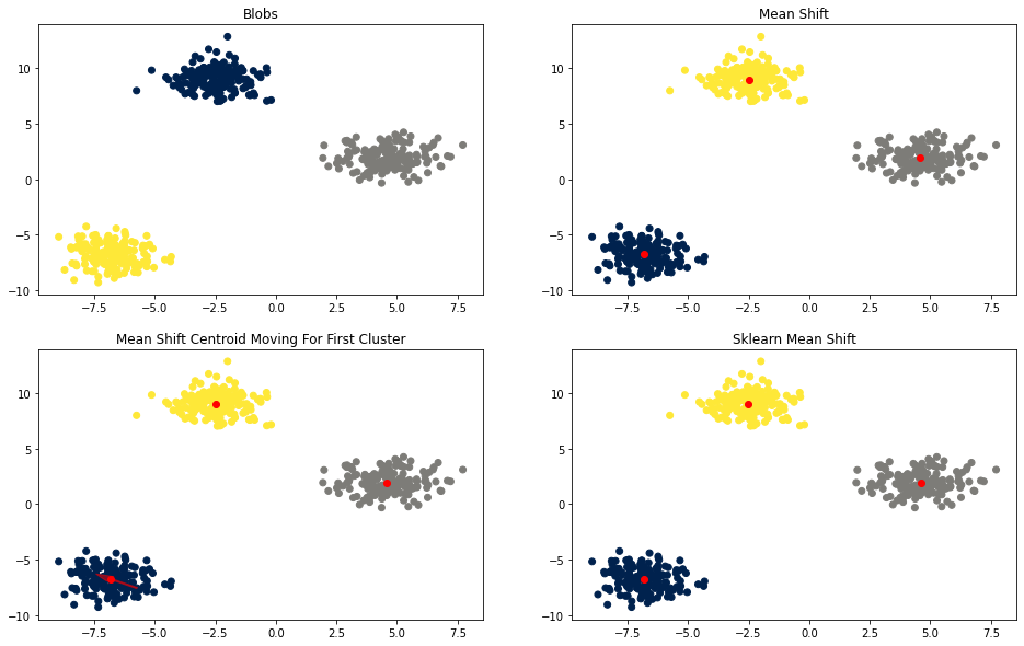
fig, axes = plt.subplots(2, 2, figsize=(16, 10))
plot_scatter(axes[0, 0], X, y, [], 'Blobs')
plot_scatter(axes[0, 1], X, labels, means, 'Mean Shift')
plot_scatter(axes[1, 0], X, labels, means, 'Mean Shift Centroid Moving For First Cluster')
plot_scatter(axes[1, 1], X, sk_ms.labels_, sk_ms.cluster_centers_, 'Sklearn Mean Shift')

plot_track(axes[1, 0], X[labels==0], means_track)
4. References
-
Dorin Comaniciu, Peter Meer(2002). “Mean Shift: A Robust Approach toward Feature Space Analysis”.
-
José E. Chacón, Tarn Duong(2018). “Multivariate Kernel Smoothing and Its Applications”.
-
M. Herbin, N. Bonnet, and P. Vautrot(1996). “A Clustering Method based on the Estimation of the Probability Density Function and on the Skeleton by Influence Zones. Application to Image Processing”.